Vol. 3 - Why Your RAG Retrieval is Failing -Search, Ranking & Retrieval Architecture

Series: Building Production RAG

In the previous article we saw how chunking strategies and embeddings shape retrieval before a single query is ever run. That was the representation layer: how the corpus is cut and turned into vectors. This article is the retrieval layer and a note on scope before we start. In Article 1, “retrieval” meant the narrow decision of whether to fetch anything at all. From here on, retrieval means the full pipeline that finds, ranks, and delivers the right chunk: storage, search, fusion, reranking. That pipeline is where things break.

Why retrieval is fast: storing is not the same as searching

Before any of the machinery, one distinction does most of the work, and it is the one people skip: storing vectors and searching them are different problems.

Storing is easy. Embed your fifty thousand documents, and you have fifty thousand vectors sitting in memory or on disk. That is a store. It keeps the data. It does nothing to help you find anything in it.

Now a query arrives, embedded into its own vector, and you want the handful of stored vectors closest to it. The obvious method is to compare the query against every stored vector and keep the nearest. That works, and it is correct, and it is linear: fifty thousand comparisons for fifty thousand documents, five million for five million. Double the corpus, double the time. This is brute-force search, and at scale it is far too slow to put in front of a user.

An index is the structure that avoids the scan. Instead of storing the vectors as a flat list, you arrange them by proximity ahead of time, so that a search can navigate toward the nearest ones rather than checking all of them. A good vector index answers a nearest-neighbour query in roughly logarithmic time: the corpus can grow by a factor of a hundred and the search slows by a little, not a hundredfold. That single property is what makes retrieval feel instant whether your corpus has ten thousand documents or ten million.

The analogy is a textbook. The pages are the store, and every word is in there. The index at the back is extra structure that lets you jump straight to “firewall, page 212” instead of reading all five hundred pages to find it. Same information, arranged for fast lookup. Take the index away and the information is still all present, but finding anything means reading the whole book.

This is why “just put the embeddings in a database” is not a retrieval system. Storage alone gives you brute-force search. The index is what buys the speed, and it is not free: building it takes time, it consumes memory, and (as we will see) it trades a little accuracy for that speed, which is why the good ones are approximate nearest-neighbour indexes rather than exact ones. Everything in the rest of this article, HNSW, the accuracy trade-off, the cost of filtering a graph, is a consequence of this one decision to index rather than scan.

It is also the quiet foundation under a claim the rest of this series leans on: that retrieval is cheap, a matter of milliseconds, while generation is the slow and expensive step. Retrieval is cheap because the embeddings were computed once at ingestion and the index lets a query skip almost the entire corpus. Take away the index and that sentence stops being true.

Storing the chunks — the vector DB

The chunks now have to live somewhere. With 50,000 documents spanning more than 100 product lines, each with three to five active versions, “somewhere” is millions of chunks -and where you put them is not an afterthought.

Retrieval is not a lookup by key or a WHERE clause, it is a similarity search. Similarity search means given a query embedding, find the chunks whose embeddings sit closest in vector space. A vanilla relational database can hold a vector (as an array or blob) but it cannot index it . Its index types (B-tree, hash) are built for exact matches and ranges, not for nearest-neighbour in high-dimensional space. So a similarity query degrades to a brute-force scan over every vector which is fine for a few thousand chunks but unusable at millions. This is the reason the vector DB exists: an ANN search -an indexstructure (HNSW, IVF, LSH…) that makes that search sublinear.

The raw vectors are the data; the HNSW graph is the index over that data.

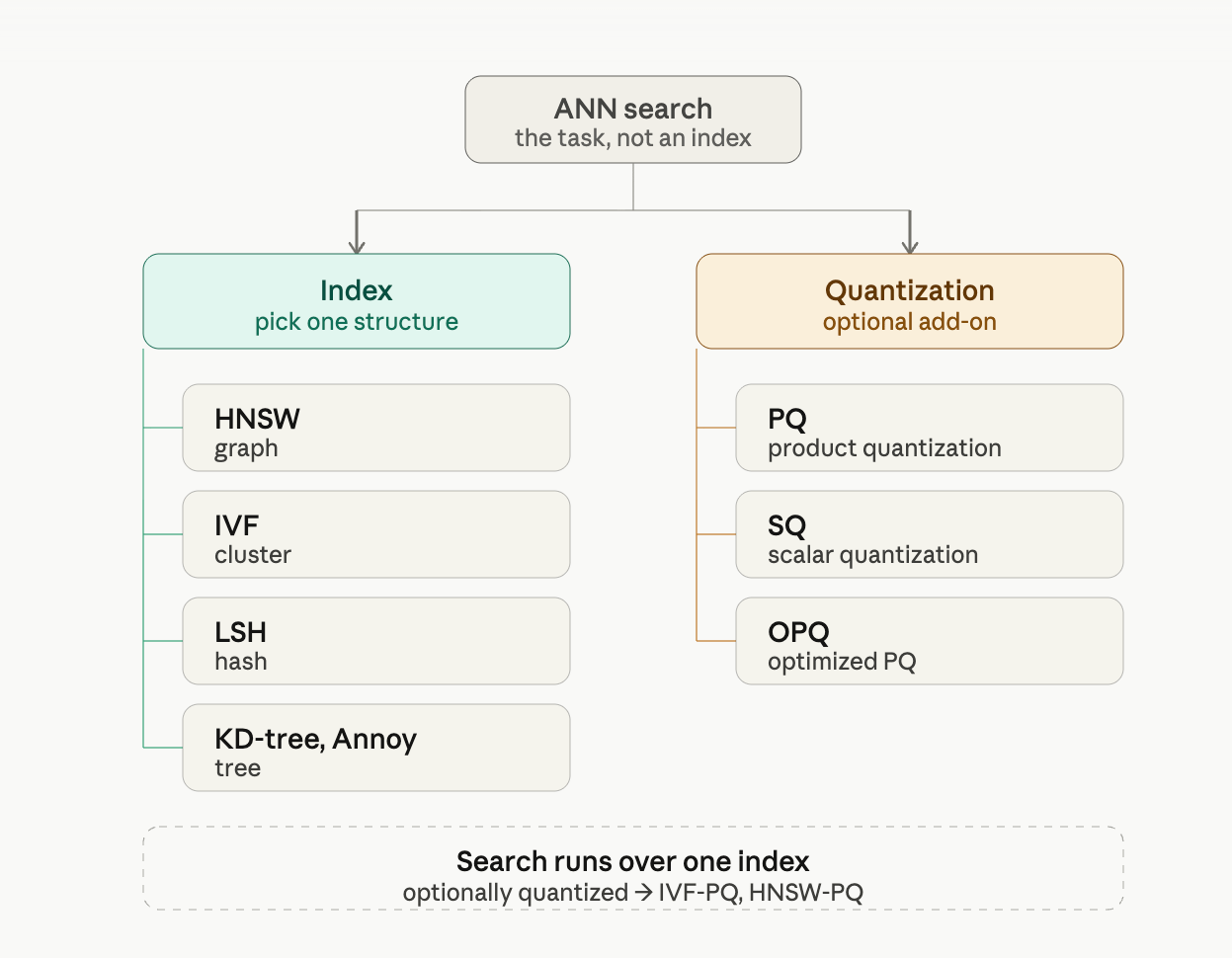
The real dividing line is the index, not the database label. That’s why pgvector, by adding ANN indexing to Postgres, makes a relational engine capable of the same job. Capable, not equivalent: a dedicated vector DB still wins on scale, native hybrid search, and peak latency. The honest call is to run the Postgres you already have until scale or native hybrid retrieval pushes you to a specialist.

The decision.

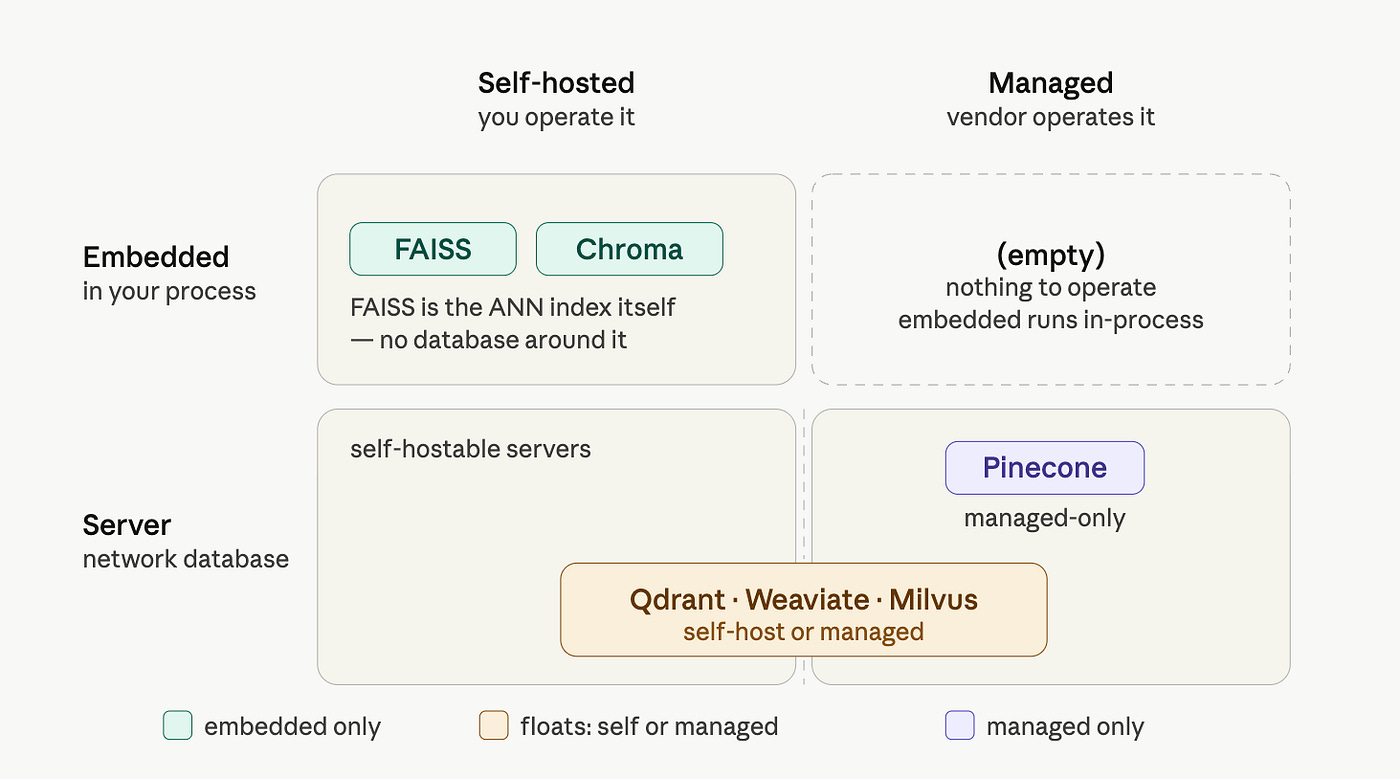
Vector stores sit on two axes, not one spectrum.

Form factor: a) embedded, running in your own process — FAISS (literally just the ANN index from above, no database around it) and Chroma — b) standalone server you query over the network.

Ownership: a) self-hosted, which you operate, b) managed, run for you by a vendor. (“Cloud” is a location, not a category — you can self-host in your own cloud.) Pinecone lives in one cell only: server, managed-only. FAISS and Chroma are embedded, so self-operated by definition. The interesting group — Qdrant, Weaviate, Milvus — is open-source and self-hostable and sold as managed cloud, which is why the same tool, Qdrant, lands in either ownership bucket depending purely on how you run it.

How it searches.

The naive approach is exact nearest neighbour (KNN) compare the query against every stored vector. Correct, but at millions of chunks it is far too slow for interactive use. Vector DBs instead use Approximate Nearest Neighbour (ANN) search, most commonly over an HNSW index (a layered small-world graph). The sparse top layers make coarse, long-range jumps to the right region of the space; the denser lower layers refine that to the actual nearest neighbours; the bottom layer holds everything. Greedy graph traversal, not a tree drill-down.

What breaks.

ANN search is approximate; that is the trade you accept for speed. It can silently miss the correct chunk. HNSW index exposes this through two parameters: M (set at build time, capping how high recall can reach) andefSearch(turned per query, deciding how much of that ceiling you actually realise) . Tune efSearch toward recall and latency climbs. Tune it toward speed and the right chunk may never enter the candidate set, and nothing downstream can recover a chunk that retrieval never surfaced. Reranking can only reorder what it was handed; generation can only synthesise from what it was given. This is the ANN index’s failure mode, and it is invisible from the outside: the answer is just quietly wrong.

Metadata and the filtering trap. Store metadata alongside each chunk and embedding : product line, version, document type. Its objective is to get precision in results, not speed: when an engineer on v4.2 asks why authentication fails, version metadata is what keeps you from returning the v3.8 procedure that is three releases stale.

But filtering is a known sharp edge on a graph index. HNSW finds things fast because of its connectivity : nodes are linked into a navigable graph, and search hops along those links. Pre-filter on “only consider chunks where version = 4.2“ and you throw away most nodes before searching. The discarded nodes were also the bridges the graph used to navigate; remove enough of them and the survivors are no longer well-connected. The search can’t hop to where it needs to go, so it returns worse results — or falls back to slow brute-force over what’s left. You filtered for precision and accidentally degraded recall or speed.

The practical resolution, which good vector DBs implement, is that how you filter matters. Pre-filter (restrict first, then search — risks breaking connectivity). Post-filter (search first, then drop non-matches — risks the top-k being entirely filtered away). Or integrated filtering (the index handles it natively, filter inside the traversal: walk through non-matching nodes but only return matching ones). Which one is right is query- and DB-dependent. In short: metadata filtering is good and you want it; the warning is against treating it as a costless, always-on first step, because on a graph index done carelessly it can quietly hurt the very recall you were trying to protect.

One property to note before the next stage: some vector DBs hold both an inverted index (for exact term match) and an HNSW vector index (for semantic match) over the same corpus. That dual capability is what makes the next decisions — HyDE, then hybrid search — possible.

Fixing the query before you search — HyDE

Unlike the stages around it, HyDE is optional — a fix you reach for when you’ve diagnosed a specific failure, not a step every query runs. The failure it fixes is a subtle asymmetry in dense retrieval: a question does not look like its answer. “Why does authentication fail after the v4.2 setup guide?” and the actual passage documenting the fix share very little surface form, so in embedding space they can land further apart than you would like. You are searching with the wrong shape of text.

HyDE — Hypothetical Document Embeddings — fixes this by transforming the probe. At query time, you ask an LLM to generate a hypothetical answer to the user’s question — a short passage that reads like the documentation you are hoping to find. You embed that hypothetical passage and use its embedding as the search vector. Because the hypothetical looks like a real answer, it lands in the right neighbourhood, and the real chunks retrieved from that neighbourhood are what you actually use.

The hypothetical is disposable. It is never stored, never indexed, never shown to the user, and it does not matter if it is factually wrong — it exists only to point the search at the right region of vector space. The grounding still comes entirely from the real chunks you retrieve.

What breaks, and when to skip it. HyDE is not free. It adds an LLM call before every search , latency and cost on the critical path of every query, just to produce the probe. And it can make things worse, not merely slower: a confidently wrong hypothetical sends the search to the wrong neighbourhood, so you spend a model call to retrieve confidently-wrong chunks. On queries where dense retrieval was already landing fine — short keyword lookups, exact identifiers, users who already phrase things like the docs — HyDE is pure downside, and the sparse side of hybrid search often covers those cases anyway. Note the scope too: HyDE reshapes the dense probe only, it does nothing for the sparse side, which still matches on the literal query. So reach for it when you’ve confirmed the surface-form gap is hurting recall, not by default.

Searching two ways at once — hybrid search

HyDE sharpened the dense probe. But dense retrieval has a blind spot no probe can fix: it matches meaning, not letters. Ask for error code AUTH_4012, or “the rate limit for API v3.2”, and dense search returns passages that are semantically adjacent -about authentication, about rate limits -while it can miss the one chunk that contains the exact token. Embeddings smear precise identifiers into their neighbourhood; that is what makes them good at paraphrase and bad at exact strings.

Sparse retrieval (BM25) has the mirror blind spot: it matches terms, not meaning. It nails AUTH_4012 because the literal token is in the index, but “reset my login” and “authentication token refresh” share no words, so it misses the paraphrase that dense would have caught.

Neither alone is enough -and that is the resolution of the BM25-vs-dense tension from Article 2. You don’t choose. You run both. This is where the vector DB’s dual-index property earns its place:

• Dense side. The HyDE-sharpened (optional) query embedding searches the HNSW vector index. The vectors hold the data; the index makes finding them fast.

• Sparse side (BM25). No embeddings exist here. The inverted index maps each term to the chunks containing it, plus frequency statistics derived from the text. The literal query matches against that , which is why HyDE doesn’t touch this path.

• Shared. The chunk text and metadata are stored once, indexed two ways.

Each retriever returns its own top-k. You now hold two ranked lists for the same query. Merging them is the next problem -and it is harder than it looks.

Merging the two lists — RRF

The problem it solves. The naive move is to add or average the two lists’ scores. But the scores are incomparable: dense gives cosine similarities (bounded, roughly 0–1), sparse gives BM25 scores (unbounded, corpus-dependent, anywhere from 8 to 30). Add them and BM25’s larger numbers dominate; normalise them and you’ve built something fragile and corpus-sensitive. The scales don’t share a meaning.

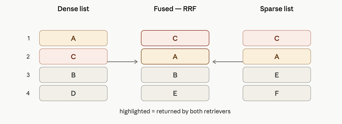
The move. Reciprocal Rank Fusion throws the scores away entirely and uses only rank -position in each list. Rank is comparable across any two systems: “position 1” means “this retriever’s best pick,” whatever the underlying score was. By discarding magnitudes, the incomparability problem disappears.

The formula. For a document d, sum a reciprocal contribution from each list it appears in:

RRF(d) = Σ  1 / (k + rank_i(d))
         i

rank_i(d) is d‘s 1-indexed position in list i; if d isn’t in list i, that term contributes nothing. k is a constant, conventionally 60.

Worked example. Two top-5 lists, k = 60:

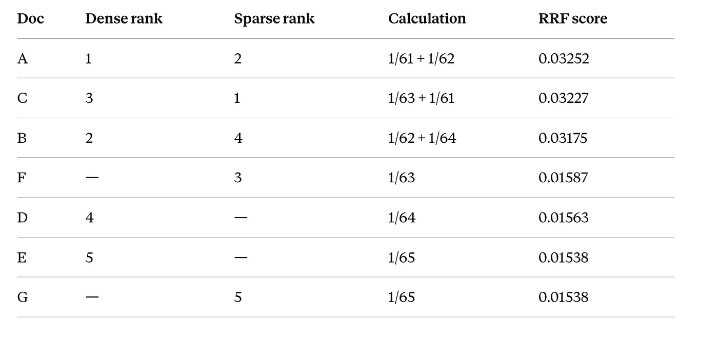
Fused ranking: A, C, B, F, D, E, G.

Read what happened. The top three -A, C, B -are exactly the documents that appeared in both lists. F is ranked 3rd by sparse, higher than B’s sparse rank of 4, yet F lands below B in the fusion. Why? B got two reciprocal contributions; F got one. RRF rewards consensus: a document both retrievers surface beats one that a single retriever ranks highly but the other never returned. That is precisely the property you want from hybrid search — agreement across two different retrieval mechanisms is a stronger signal than enthusiasm from one.

What k does. Notice every contribution sits between 1/61 and 1/65 -nearly identical. At k = 60, within-list rank barely matters; what dominates is how many lists a document appears in. Drop k toward 0 and the gaps explode-at k = 0, rank 1 contributes 1.0 and rank 2 contributes 0.5, so the top of each list dominates everything. Raise k and contributions flatten further, leaning even harder on cross-list agreement. So k is the dial between “trust the top of each list” (small k) and “trust agreement across lists” (large k). 60 is a moderate default that leans toward consensus — usually what you want, but a knob, not a law.

Reordering for true relevance — reranking

RRF hands you one fused list ordered by rank-consensus. But rank-consensus is a coarse signal, it knows position, not true relevance to this specific query. And recall the bi-encoder limitation from Article 2: query and chunk were embedded separately and compared by cosine, so they never actually interacted. That separation is what makes first-stage retrieval fast , chunks are pre-embedded and also what makes it blunt.

A cross-encoder fixes the bluntness. It takes the query and a chunk together in a single forward pass, with full attention between them, and outputs a relevance score directly. It produces no embedding , it can’t, because the score depends on the pair, not on either piece alone. That is exactly why it can’t be precomputed, and exactly why it is accurate: the model sees how this query relates to this chunk, word by word.

The cost is that you cannot run it over the corpus. So the pattern is two-stage by necessity: retrieve broad, rerank narrow. Hybrid search plus RRF gives you a fused candidate set let’s say the top 50. The cross-encoder scores those 50 and you keep the top 5. A cheap, wide first stage; an expensive, precise second stage.

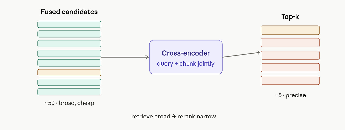
What breaks. Latency and cost scale with how many candidates you rerank. Rerank 500 and you have reintroduced the very slowness ANN was built to avoid. The dial here is the candidate-set size: wide enough that the right chunk is reliably inside it, narrow enough that the cross-encoder stays affordable. Too narrow and you defeat the broad-recall first stage; too wide and you defeat the point of approximate search upstream.

Delivering the right chunk — parent-child

One last decision, and like HyDE, it is optional. You need it only when the unit that searches well isn’t the unit that answers well. Small chunks retrieve precisely: a tight, single-topic chunk has a sharp embedding, so search lands on it cleanly. But that same small chunk is often too thin for the LLM to answer from, it found the right spot without enough surrounding context. When searching and answering want different sizes, parent-child splits them: you embed and search the small unit (the child), but return the larger unit it sits inside (the parent) to the LLM. If your chunks are already sized to do both jobs, you skip this entirely.

Mechanically this is a two-store split. The vector DB holds the embedded children; a separate docstore (a plain key-value store) holds the raw parent text. Parents are never embedded , only fetched by key and each child carries a pointer to its parent. At query time you search children, follow the pointers up, dedup to the distinct parents, and pass those to generation.

The docstore is a role, not a product, back it with whatever fits your scale. The default InMemoryStore keeps every parent in process RAM and vanishes on restart, which is fine for a notebook but a memory-and-durability liability at 50,000 documents. A LocalFileStore moves parents to local disk. A RedisStore puts them in a separate Redis process that persists and can be shared across app instances. Reach for one of those the moment it’s something you intend to keep , the InMemoryStore default is the trap most first implementations ship.

The chunk is in the window — now what?

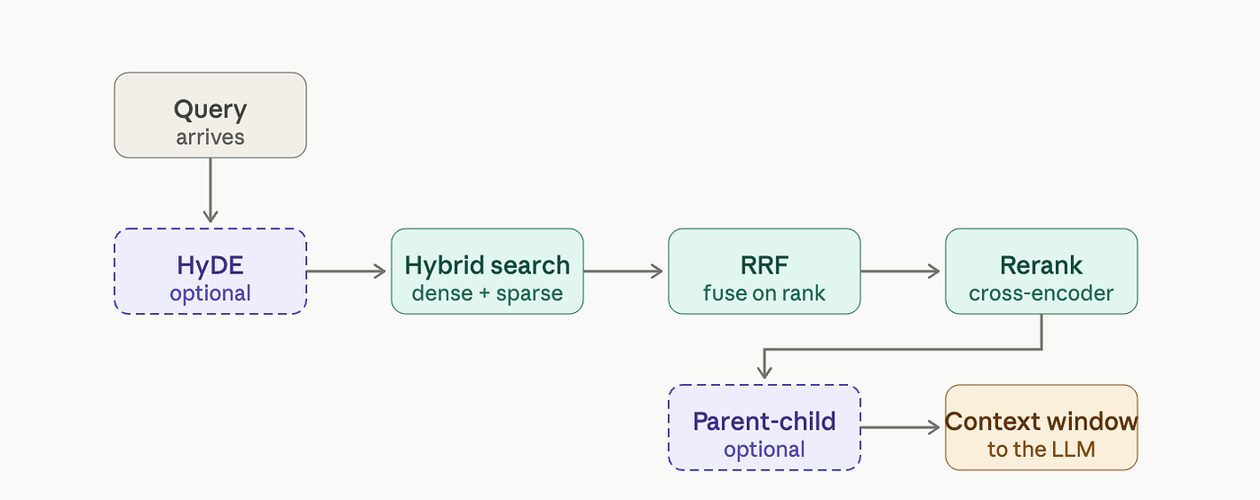
Trace the journey: the query arrived, HyDE reshaped the dense probe, hybrid search ran both retrievers, RRF fused them on rank, the cross-encoder reranked the candidates, and parent-child delivered the right context at the right size. The correct chunk is now in the LLM’s context window.

But retrieval ends here, and a perfect chunk is not a perfect answer. Drop the right context into a careless prompt and the model still produces a bad response , the right facts, badly framed, or buried, or contradicted by a worse chunk sitting next to them. That is augmentation and generation: the A and the G of RAG, and the subject of the next article.

Next in the series: Why Your RAG Generation is Failing -Augmentation, Prompt Construction & Synthesis.